How to Split Cells in Excel?

Microsoft Excel allows you to organize and manipulate data in various ways. When dealing with large datasets or information that needs to be segmented, the ability to split cells becomes a valuable tool. Splitting cells in Excel involves dividing the content of a single cell into multiple cells, which can be especially useful when you need to separate names, addresses, or other pieces of data currently combined in one cell. Learn how to split cells in Excel using built-in Excel functions and formulas.

Splitting in Excel is very simple. If you have multiple values in a single cell and want to separate them across multiple cells, Microsoft Excel has some easy-to-use options. This guide explores the techniques and methods for splitting cells in Excel, enabling you to efficiently manage and structure your data for better analysis and presentation.

Content

• Split Cells using Text to Columns
• Split cells in Excel diagonally
• Flash Fill to Split Cells
• Excel text functions to Split Cells

How to Split Cells using Text to Columns

The easiest way to split cells is using the Text to Columns function. Let's check how to split a cell diagonally in Excel.

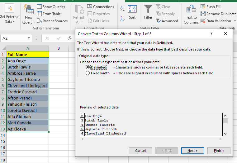
Below are some names we need to break into two parts.

• Select all the cells that you want to split.
• Locate Data ⇒ Data Tools ⇒ Text to Columns.

• A Convert Text to Columns wizard will pop up. Choose the file type that is relevant to your data. In this case, we will choose Delimited.

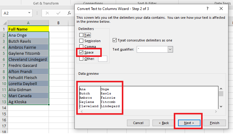
• In the next step, we will select the delimiter for our data set. Since Space separates the names, we will select Space. Depending on what delimiter the data set has, choose your option. In the data preview, you can see how the cell will be split.

Press Next to set the data format. Select General if you don’t want to apply any other advanced settings. 

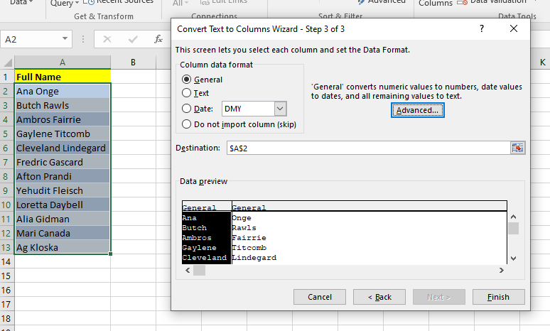
You can choose Advanced Settings if you are working on numeric data and want to recognize numeric data.

Since we don’t want to use additional settings, we will click Cancel and Finish while selecting General. 

The cell has now split into 2.

Split Cells Diagonally

We have already seen how to split a cell in Excel and its contents. Next, we will teach you how to split an Excel cell diagonally. Don’t worry, it’s very simple. Just follow these steps:

Step 1. Select the cell you want to split diagonally, right-click and choose the Format Cells option, as the following image illustrates.

Step 2. In the dialogue box, go to the Border tab and click the button containing the diagonal artwork, and then click OK.

Once you’ve clicked OK, we’ll have our cell divided diagonally. 

Next, highlight the first word and go to the Fonts tab located in the Home tab’s bottom corner of the Fonts group.

In the dialogue box, check the Superscript box and click OK. Then, repeat the same procedure for the other word, but you will put the Subscript option on this one and click OK.

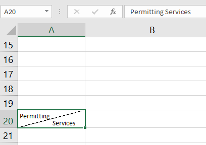
As you can see, the two words are now split diagonally in the cell.

Flash Fill for Splitting Cells  

You must know this commonly used Excel function. You must tell Excel how you want your data to split in flash fill.

We will go to –

Data ⇒ Data Tools ⇒ Flash Fill

Now, follow the same process for the next part of the string.

Excel Text Functions for Splitting Cells 

You can split a cell in Excel using different text functions. These text functions allow you to extract parts of a cell that you can send to another cell.

Text functions in Excel include:

• Left() – To extract several characters from the left side of the text
• Right() – To extract multiple characters from the right side of the text
• Mid() – To extract multiple characters from the middle of a string
• Find(): To find a substring within another string
• len() – It returns the total number of characters in a text string
• All these functions are not required to split cells, but there are specific ways you can use them in formulas to achieve the results.

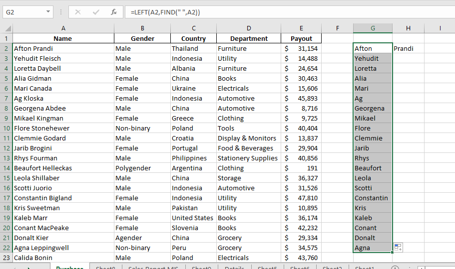
For example, you can extract the name from the Left and Find function. The Find feature helps because it can tell you where the delimiter character is. In this case, it is a space.

So the function would look like this:

=LEFT(A2,FIND(” “,A2))

When you press enter after typing this formula, you will see that the first name is extracted from the string in cell A2.

This works because the Left function needs the number of characters to extract. Since the space character is placed at the end of the name, you can use the LOOKUP function to find the space, which returns the number of characters you need to get the name.

You can extract the last name using the Right or Middle functions.

To use the Right function:

=RIGHT(A2,LEN(A2)-FIND(” “,A2))

This will extract the last name by finding the position of the space and then subtracting it from the total string length. This gives the Right function the number of characters it needs to extract the last name.

You can now drag the formula to the rest of the cells.

Splitting cells in Excel offers a versatile way to organize your data and improve readability. You can efficiently structure your Excel sheet by choosing the correct method between Text to Columns, formulas, or Flash Fill. Mastering these techniques will save you time and improve the accuracy of your work. Remember to consider the nature of your data and desired outcome when selecting your splitting technique.

Hope this article was helpful.

Top Trending Articles in MS Excel:

Most Useful Excel Formulas | Min Max Functions in Excel | Average Functions in Excel | Introduction to MS Excel | Financial Modelling in Excel | MS Excel interview questions | Sum Function in Excel | Trim Function in Excel | Pivot Table in Excel | Percentage in Excel | Vlookup in Excel | Median Function in Excel | Types of Charts in Excel | Count Function in Excel | MS Excel Vs. Google Sheet | Remove Duplicates in Excel | Create Graph in Excel