
What is Filter in Excel: How to Use Them?
In Excel, a filter is a powerful tool that allows users to display only the data that meets specific criteria, making it easier to analyze and manage large datasets. Filters can be applied to a range of data or an entire table, enabling users to hide rows that do not match the selected criteria while keeping relevant information visible. In this article, you will learn how to use filters in Excel.

The filter in Excel is an essential tool for displaying relevant data. It temporarily eliminates irrelevant entries from the view. This tool filters data according to criteria to help analyze critical data points. The article discusses the topic: What is Filter in Excel?
Enhance Your Learning: To improve your data analysis skills, we recommend you take online data analysis courses or consider FREE online courses from top online course providers such as edX, Udemy, Coursera, Alison, Futurelearn, etc.
Content
- How To Use Filters In Excel
- Excel Filters Options
- Filter By Multiple Columns
- How To Remove A Filter In Excel
- Types of Filters in Excel
- Keyboard Shortcuts for Filters in Excel
Filter Data in an Excel Table
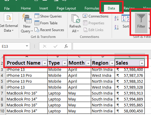
The Filter button is located in the ribbon. You can find the Filter command –

When you press the Filter button, you will see that the data range headers have arrows, indicating that the dataset is ready to use filters.
If you want to boost your data analytical skills then start with learning MS Excel! We recommend you to select the most suitable MS Excel online courses as per your professional and personal goals. Learn how to use both basic and advanced Excel formulas and functions, dashboards, macros, pivot tables, and data analysis tools to improve business insights and reporting.
How To Use Filters In Excel?
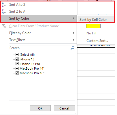
We must choose a column to filter the information and click the corresponding filter arrow to display the filtering options. At the bottom, all filters will display a list of unique values with a checkbox to the left.

In the above screenshot of the dataset, you can see that when we click on the arrow icon in the Product Name header, a drop-down menu allows us to select the product for which we want to check the data.
Best-suited MS Excel courses for you
Learn MS Excel with these high-rated online courses

Excel Filters Options
The Excel filtering options of the headers are presented to us with a dialogue box or options box allowing us to do various operations. These filter options are categorized into three segments –
Sort Options:
- Sort from A to Z (or from highest to lowest if numeric)
- From Z to A (or smallest to largest if numeric)
- Sort by color (custom option)
Must Explore – Free MS Excel Courses
Filter Options
- Clear Filter From (Heading Name)
- Filters by Color
- Text filters

Explore MS Excel Courses
Selection Panel
- Search bar
- Multiple selection list for quick filters
Filter a Database in Excel
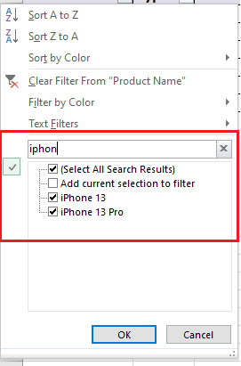
One option to filter the data is to individually choose those values we want to display on the screen. We can also use the (Select All) option to check or uncheck all items on the list. In this dataset, we have selected only the data for iPhone 13 Pro, so the filter will show only the rows where iPhone 13 Pro is mentioned.

Pressing the OK button will hide the rows that do not meet the established filter criteria. Notice that the filter arrow in the Product Name has changed to tell us we’ve applied a filter for iPhone 13 Pro. We can now see data only for iPhone 13 Pro.

The funnel sign in the header suggests that it has a filter applied.

Filter by Multiple Columns
If we want to segment further the data displayed on the screen, we can filter it by several columns. In the previous example, I filtered the rows belonging to iPhone 13 Pro. Still, if I also need to know which ones belong to the West and North regions, then I must select these options within the Region column filter, selecting the data for West.
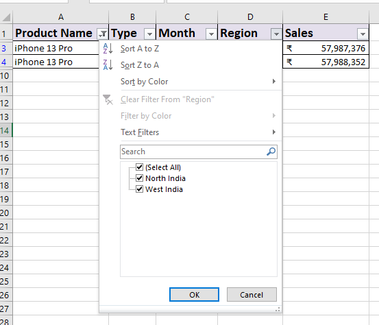
Accepting these changes will display only the rows that meet both criteria. Note that both columns will have changed their icons to indicate that a filter has been applied to each.

This example shows that it is possible to create as many filters as there are columns in our data, and the more filter criteria we apply, the greater the data segmentation we will obtain.

 Read Later

How to Remove a Filter in Excel?
To remove a filter applied to a column, we must click on the filter arrow and select the Clear option filter from “Column,” where Column is the name of the column we have chosen.

This action will remove the filter from a single column, but if we have filters applied to several columns and want to remove them all with a single action, we must press the Clear command found in the Data ⇒ Sort and filter.


Types of Filters in Excel
When we have a massive list of unique values and can’t quickly identify the ones we want to select, we can use the search box to find the values we need. You can also use wildcard characters such as the asterisk (*) or question mark (?) just as if we were doing a fuzzy search in Excel so that we can broaden the search results.
Text Filters In Excel
Apart from the options already mentioned to filter in Excel, when the text data type is detected in a column, a menu option called Text Filters will be displayed like the following:
- When choosing any of these options, a dialog box will be displayed to allow us to configure each available criterion. For example, choosing the Begins With option will display the following dialogue:
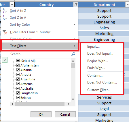
- If we put the letter “a” in the text box next to the “begins with” option, then Excel will show only the items in the Country column that start with the letter “a.”

- If you want to be more specific and select a particular country, then uncheck Select All.

- Select the country for which you want to check the data. For example – we have checked Afghanistan here.


Similarly, you can uncheck the boxes for the values for you do not need data.

Number Filters In Excel
Similarly, suppose Excel detects that a column contains numerical values. In that case, it will allow us to use specific filters for that data type, as you can see in the following screenshot.

Unlike the Text Filters, Excel will allow us to use the Number Filters to show values greater than or equal to another or simply those greater than the average, Top 10, and even custom filter.

Date Filters In Excel
Dates are the type of data that provide us with the most filtering options, as shown in the following image:

You can select the data year-wise, month-wise, and day-wise. In the example below, we unchecked Select All and just clicked 24 inside the August month data.

Now I can see only the data for August 24, 2022.

Filter By Color In Excel
We can also filter the data by Color, as discussed above. To enable this option, the cells must have a fill color applied either by a conditional formatting rule or by directly modifying the fill color with the formatting tools. In our example, we have applied the Conditional Formatting option for cells containing employee data above PayGrade 15.

You can see that the cells with numbers more than 15 are colored yellow. Now you can Filter by Color.


Keyboard Shortcuts for Filters in Excel
MS Excel Filters can also be applied using keyboard shortcuts. Check them out -
| Action |
Shortcut (Windows) |
Shortcut (Mac) |
Description |
| Apply or Remove Filters |
Ctrl + Shift + L |
Command + Shift + F |
Toggles filters on or off for the selected table or range. |
| Open Filter Dropdown Menu |
Alt + Down Arrow |
Control + Option + Down Arrow |
Opens the filter dropdown menu for the active cell. |
| Clear Filters from a Column |
Alt + Down Arrow + C |
Use filter menu manually |
Clears filters applied to the current column. |
| Select Filter Criteria |
Use Arrow Keys + Space |
Use Arrow Keys + Space |
Navigate and select/deselect checkboxes in the filter dropdown menu. |
| Filter by Cell's Value or Color |
Alt + Down Arrow + F |
Use filter menu manually |
Opens options to filter by the selected cell's value or color directly from the dropdown menu. |
| Move to the Next Filter Column |
Tab |
Tab |
Moves focus to the next column with a filter applied. |
| Move to the Previous Filter Column |
Shift + Tab |
Shift + Tab |
Moves focus to the previous column with a filter applied. |
| Remove All Filters |
Alt + D + F + F |
Use filter menu manually |
Clears all filters applied across the worksheet. |
You can now see the data coded Yellow.
Hope it was fun to learn about using Filters in Excel. Try your hands on the data sets to understand the functions better.
Top Trending Articles in MS Excel:
Most Useful Excel Formulas | Min Max Functions in Excel | Average Functions in Excel | Introduction to MS Excel | Financial Modelling in Excel | MS Excel interview questions | Sum Function in Excel | Trim Function in Excel | Pivot Table in Excel | Percentage in Excel | Vlookup in Excel | Median Function in Excel | Types of Charts in Excel | Count Function in Excel | MS Excel Vs. Google Sheet | Remove Duplicates in Excel | Create Graph in Excel
FAQs
What does Filtering data in Excel mean?
Filtering data in a spreadsheet means setting conditions to display only specific data. It makes it easier to focus on certain information in a large data set or data table. Filtering does not remove or change the data; it simply modifies which rows or columns to display in the active Excel spreadsheet.
What are the types of filters in Excel?
Excel includes two types of filters - Automatic filter: It shows us all the information regarding the criteria we are looking for, be it text, number, date, color, currency, etc. Advanced Filter - it extracts information regarding more personalized criteria. Usually, the information that you want to extract is used for reports.
How to filter numeric data in Excel?
Numeric data can be filtered based on: If the data is equal to a certain number. Whether the data is greater than or less than a specific number. The data is above or below the average value of the data. Filter text data
How to filter text data?
Text data can be filtered based on: If the data matches a given word. If the data is a word containing one or more letters. If the data is a word that begins or ends with a specific alphabet letter.
What should I do if the Filter option is not working in Excel?
If the filter is not functioning, please follow these steps:
- Make sure you have no blank rows or columns in your dataset.
- Ensure headers are properly formatted.
- Check if the worksheet is being protected, as filters do not apply to protected sheets.
- Delete and reapply the filter by going into the "Filter" button on the "Data" tab.
Can I filter data based on color in Excel?
Yes, Excel supports filtering by color.
- Select the filter drop-down arrow.
- Select "Filter by Color" and the desired color.
- Excel will show you only rows with the specified color.
Can I filter numbers and text separately?
Yes, Excel provides different filtering options:
- For numbers, you can filter by conditions like Greater Than, Less Than, Between, or Equals.
- For text, you can filter by Contains, Begins With, Ends With, or Equals.
Can I filter data by multiple columns in Excel?
Yes, you can filter for more than one column. Put a filter on one column, and then do the same for another column. Excel will show only the rows that match all the filters applied.
What is the difference between AutoFilter and Advanced Filter?
- AutoFilter: A quick filter option that enables users to filter data on chosen criteria.
- Advanced Filter: A more advanced tool allowing users to create complex filtering conditions, like filtering data on multiple criteria through a separate range.

Rashmi Karan is a writer and editor with more than 15 years of exp., focusing on educational content. Her expertise is IT & Software domain. She also creates articles on trending tech like data science,